Proper Acceleration - The Electromagnetic Nature Of ThingsThe Electromagnetic Nature Of Things

Jan Onderco

March 2023

Abstract

The proper acceleration is absolute, an accelerometer measures one and only one value at a point in space and time. An accelerations of combined two circular motions are being investigated using generic motion equations. Trajectory curvature radius is a primary factor in acceleration analysis and determines the absolute acceleration. Inertial observers in a relative motion do not agree on trajectory curvature radius, that makes the acceleration covariant, frame dependent. The logical conclusion is an existence of an absolute reference frame where only one absolute acceleration analysis is true, providing correct prediction for the absolute acceleration.

Introduction

The general motion acceleration analysis can be found in many textbooks.^[1]

Figure 1: General motion of a rigid body in space where reference axes origin attached to B translates and rotates with angular velocity $\boldsymbol{\Omega}$ in reference to origin $O$ . The angular velocity $\boldsymbol{\Omega}$ may differ from body angular velocity $\boldsymbol{\omega}$ .

The generic motion equations for velocity and acceleration of point $A$ as per Figure 1 are

$\boldsymbol{v}_A =\boldsymbol{v}_B+\boldsymbol{\Omega} \times \boldsymbol{r}_{A/B} + \boldsymbol{v}_{rel}$
$\boldsymbol{a}_A =\boldsymbol{a}_B+\boldsymbol{\dot{\Omega}} \times \boldsymbol{r}_{A/B}+\boldsymbol{\Omega} \times (\boldsymbol{\Omega} \times \boldsymbol{r}_{A/B})+2\boldsymbol{\Omega} \times \boldsymbol{v}_{rel} + \boldsymbol{a}_{rel}$

The acceleration equation represents our current understanding of general motion and it captures the ultimate case when the reference axes attached to point $B$ rotate as well as translate. The acceleration analysis follows for a simple mechanical ‘spin-orbit simulation’, a combination of two rotations as shown in Figure 2.

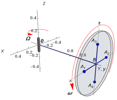
Figure 2: Spinning flywheel mounted on a rotating arm that generates flywheel ‘orbit’ around the origin $O$ of $X, Y, Z$ inertial reference system. Point $B$ is the flywheel center of mass and points $A_1, A_2, A_3, A_4$ represent center of mass of four ‘pie’ flywheel symmetrical cut-outs.

A spinning flywheel is mounted on a rotating arm that generates flywheel ‘orbit’ around the origin $O$ of $X, Y, Z$ inertial reference system with unit vectors $\{\boldsymbol{I, J, K}\}$ . The accelerated point $B$ is the center of mass of the rotating/spinning flywheel $1m$ from the origin $O$ . The origin of $x, y, z$ (unit vectors $\{\boldsymbol{i, j, k}\}$ ) reference system is in the point $B$ and it rotates with $\boldsymbol{\Omega}$ angular velocity. The flywheel rotation is $\boldsymbol{\omega}$ . The points $A_1, A_2, A_3, A_4$ represent center of mass of four ‘pie’ flywheel symmetrical cut-outs. The first case initial values are

The velocity calculations are

The acceleration calculations are

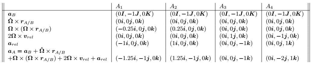
The $A$ points accelerations are a function of $\boldsymbol{\omega}$ , $\boldsymbol{\Omega}$ , the curvature radius of $\boldsymbol{\Omega}$ is the main factor appearing in multiple acceleration components. The points $A_1$ and $A_2$ have the centripetal acceleration in $-y$ direction $1m/s^2$ . The point $A_3$ does not have any centripetal acceleration in the $-y$ direction and the point $A_4$ has $2m/s^2$ in the $-y$ direction. The delta between $A_3$ and $A_4$ points causes a torque in the $-x$ direction as per Figure 3. All four $A$ points experience the centripetal acceleration towards the center of the flywheel.

Figure 3: The green arrows represent the acceleration in the $A$ points. The torque generated between $A_3$ and $A_4$ points; the red arrow starting in the point $B$ contributes to the flywheel precession.

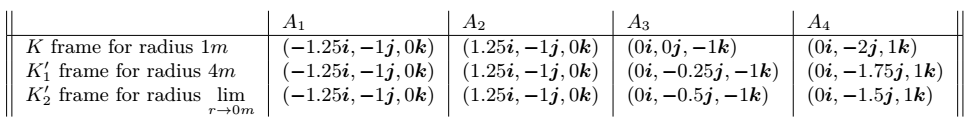
The relationship between $\boldsymbol{\Omega}$ , radius $\boldsymbol{r_B}$ is a factor influencing the $B$ and $A$ points accelerations. The following calculations maintain the same acceleration of point $B$ but $A$ points accelerations are different. The radius $\boldsymbol{r}_B=(0\boldsymbol{I},\, 100\boldsymbol{J},\, 0\boldsymbol{K})$ ; $\boldsymbol{\Omega} =(0\boldsymbol{I},\, 0\boldsymbol{J},\, 0.1\boldsymbol{K})$ ; $\boldsymbol{\omega} =(0\boldsymbol{I},\, 2\boldsymbol{J},\, 0.9\boldsymbol{K})$ and $\boldsymbol{r}_B=(0\boldsymbol{I},\, 10000\boldsymbol{J},\, 0\boldsymbol{K})$ ; $\boldsymbol{\Omega} =(0\boldsymbol{I},\, 0\boldsymbol{J},\, 0.01\boldsymbol{K})$ ; $\boldsymbol{\omega} =(0\boldsymbol{I},\, 2\boldsymbol{J},\, 0.99\boldsymbol{K})$ end up with the same point $B$ instantaneous acceleration $\boldsymbol{a}_B=(0\boldsymbol{I},-1\boldsymbol{J},0\boldsymbol{K})$ but the $A$ points accelerations differ as per the following table.

The $X, Y, Z$ inertial reference system represents a stationary grid of inertial observers in regards to the origin $O$ and we will define it as a rest frame of the spin-orbit simulation. A question arises, can we move the origin $O$ to a different observer within the same inertial observer grid? For example, can we chose $O_1=(0\boldsymbol{I}, -99\boldsymbol{J}, 0\boldsymbol{K})$ in reference to the origin $O$ so the new $\boldsymbol{r}_{B_{O_1}}=(0\boldsymbol{I},\, 100\boldsymbol{J},\, 0\boldsymbol{K})?$ If it is done then the acceleration calculation results are not the same based on the generic motion equations because $\boldsymbol{r}_B$ changed. If the desired outcome is the have the same acceleration at point $B$ then the angular velocities $\boldsymbol{\Omega} =(0\boldsymbol{I},\, 0\boldsymbol{J},\, 0.1\boldsymbol{K})$ and $\boldsymbol{\omega} =(0\boldsymbol{I},\, 2\boldsymbol{J},\, 0.9\boldsymbol{K})$ have to change but still accelerations in points $A_3$ , $A_4$ would be different when compared to $O$ origin. The accelerations at points $B$ , $A_3$ , $A_4$ are absolute and the accelerations determine the absolute angular velocities $\boldsymbol{\Omega},\,\boldsymbol{\omega}$ .^[1] The accelerations can be measured, they represent an objective reality. The curvature $\kappa=|\boldsymbol{\dot{r}} \times \boldsymbol{\ddot{r}}|/|\boldsymbol{\dot{r}}|^3$ ^[2] helps in deciding what is the true origin. The curvature $\kappa=1$ in our case therefore curvature radius is $r=1/\kappa=1$ and the true rotation origin is $O$ based on the normal and tangential coordinates^[3] (n-t) calculations.

An argument can be made the parametric equations using Cartesian/rectangular coordinates^[4] have the analysis covered properly. The point $B$ moves in the $X, Y$ plane where $(Z=0)$ and we can write $\boldsymbol{r}(t)$ , $\boldsymbol{v}(t)$ , $\boldsymbol{a}(t)$ …

An accelerated observer at point $B$ is placed in a box around the flywheel, no signal from the outside of the box and the $B$ observer has access to $A$ points acceleration measurements. Can $B$ observer recover velocity, position equations from the acceleration all the way to $a, b$ constants or that information is lost/hidden to the $B$ observer?

The $B$ observer measures acceleration $1m/s^2$ at $B$ location. Is it a curved acceleration with some $\boldsymbol{r}, \boldsymbol{\Omega}$ or straight line linear acceleration? The $A_3$ , $A_4$ points accelerations answer that question. The $\boldsymbol{r}, \boldsymbol{\Omega}$ and $\boldsymbol{\omega}$ are recovered, so is the curvature $\kappa$ and the $B$ observer can identify the true origin $O$ . Any other rest frame inertial grid observer will have $a, b$ position transformation. The information is not lost and it can be recovered from the inside of the box. Here, a foundation has been established for the principle, the information about the acceleration, the acceleration curvature radius, is intrinsically imprinted in the matter itself. The signal comes from the inside, it does not have to come from the outside.

Acceleration – moving inertial observers

The next step is to calculate the same ‘spin-orbit’ acceleration from moving inertial reference grid of observers. The rest frame inertial frame is named $K$ , the $K'_1$ inertial frame moves with velocity $\boldsymbol{v}=1m/s$ along the $X$ axis in the rest frame $K$ and $K'_2$ inertial frame moves with velocity $\boldsymbol{v}=-1m/s$ along the $X$ axis in the rest frame $K$ .

Figure 4: The point $B$ trajectory the moving frames is the cycloid. The $K'_1$ frame observers the point $B$ at the top/bottom of the cycloid, the $K'_2$ frame observes the point $B$ at the cusp of the cycloid.

The rectangular coordinates point $B$ acceleration analysis agrees with the (n-t) coordinates analysis in all three inertial frames. The $K'_1$ inertial frame observes $1m/s$ normal acceleration, an instantaneous pure centripetal acceleration, and the $K'_2$ frame observes $1m/s$ tangential acceleration, an instantaneous pure straight line linear acceleration, even though $K'_1$ and $K'_2$ frames do not agree on the trajectory curvature. The $K'_1$ trajectory curvature is $0.25m^{-1}$ , radius is $4m$ and the $K'_2$ trajectory curvature is infinite, radius is $0m$ , a ‘singularity/black hole’. The calculation result shown below is for radius $\lim\limits_{r \to 0}$ and not for $r=0$ .

The $A$ points accelerations (n-t) coordinates results are

Three different inertial reference frames have three different results for points $A_3, A_4$ while the frames agree on $A_1, A_2$ accelerations. The calculation steps are listed in the Appendix. If a measurement is made with $K'_1$ , $4m$ radius values at points $A_3$ , A_4$ then how does the inside observer knows it is a cycloid motion and not a circular one? The consequent $A_3, A_4$ acceleration measurement after a $dt$ would have to be constant for the circular trajectory but it would change for a cycloid. The acceleration and more specifically acceleration $dt$ changes are absolute and unique for any trajectory.

Uniform straight line acceleration

An inertial observer can become non-inertial in following ways: straight line acceleration, rotation or combination of these two instances. The previous section already showed the trajectories of accelerated particles/observers have different shapes in moving inertial frames. The $K'_1$ observer saw the rotating flywheel at the cusp and the $K'_2$ observer saw the wheel at the top of the cycloid. The straight line trajectory of the straight line acceleration in the rest frame $K$ will appear as curved trajectory in frames $K'_1$ and $K'_2$ . The $K'_1$ inertial frame moves with velocity $\boldsymbol{v}=1m/s$ along the $X$ axis in the rest frame $K$ as in the previous example and $K'_2$ inertial frame moves with the velocity $\boldsymbol{v}=-1m/s$ along the $X$ axis in the rest frame $K$ .

Figure 5: The point $B$ trajectory for the uniform straight line acceleration in the rest frame $K$ at time $t=0$ . The $B$ and $A$ points accelerations are equal in the $-Y$ axis direction.

The rotating flywheel accelerated in a straight line along $-Y$ axis direction with $1m/s^2$ acceleration in the $K$ rest frame is expected to generate equal proper acceleration in all four $A$ points. The proper absolute acceleration is expected to be measured at $A$ points by accelerometers.

The observers $O$ , $O'_1$ , $O'_2$ are aligned at time $t=0$ , the $B$ position vectors are equal $\boldsymbol{r}_{B}=\boldsymbol{r}_{B'_1}=\boldsymbol{r}_{B'_2}$ at $t=0$ . There is no $\boldsymbol{\Omega}$ in the $K$ frame but $\boldsymbol{\Omega}_{K'_1} =(0\boldsymbol{I},\, 0\boldsymbol{J},\, 1\boldsymbol{K})$ in $K'_1$ frame and $\boldsymbol{\Omega}_{K'_2} =(0\boldsymbol{I},\, 0\boldsymbol{J},\, -1\boldsymbol{K})$ in $K'_2$ frame. $K'_1$ frame observes ‘pure’ centripetal acceleration at $t=0$ , point $B'_1$ moves with velocity $\boldsymbol{v}=-1m/s$ along the $X'$ direction and $K'_2$ frame observes similar ‘pure’ centripetal acceleration but in opposite direction. The flywheel does not rotate around $Z$ axis direction, to compensate $\boldsymbol{\omega}_{K'_1} =(0\boldsymbol{i},\, 2\boldsymbol{j},\, -1\boldsymbol{k})$ and $\boldsymbol{\omega}_{K'_2} =(0\boldsymbol{i},\, 2\boldsymbol{j},\, 1\boldsymbol{k})$ in $K'_1$ and $K'_2$ frames. The $K'_1$ trajectory $Z$ axis rotation $1\boldsymbol{K}$ is cancelled by flywheel $-1\boldsymbol{k}$ , the same applies to $K'_2$ frame rotations in opposite directions.

Figure 6: The point $B$ trajectory for the uniform straight line acceleration as observed in $K'_1$ (left, orange line). The point $B$ trajectory for the uniform straight line acceleration as observed in $K'_2$ (right, cyan line). The $B$ and $A$ points accelerations are not equal in the $-Y$ axis direction.

Considering the change when the flywheel does not rotate around $Z$ axis the acceleration calculations are different compared to results where the flywheel rotates around $Z$ axis.

Only one set of values can be true in the table above. The straight line acceleration has infinite curvature radius in the (n-t) coordinates analysis. Infinity values in physics lead to singularities, discontinuations, undefined conditions, therefore the straight line acceleration does not exist. Only one inertial observer sees the straight line acceleration every other moving inertial observer sees a curved trajectory where the curvature radius is not infinity.

Equivalence Principle

Equivalence principle: as far as physical measurements are concerned, an inertial observer in a uniform gravitational field is equivalent to a uniformly accelerated observer in the absence of any gravitation field.^[5]

The straight line uniformly accelerated observer does not exist. The Equivalence Principle does not hold.

The infinity curvature radius is one disqualifier why the straight line uniformly accelerated observer does not exist. The second one is the concept of momentarily comoving observers.^[6] If the starting preferred inertial observer analysis is correct then the preferred observer does not agree with the analysis of comoving observers due to worldline curvature radius changes. The comoving observers maintain constant worldline curvature radius but the preferred inertial observer sees the worldline curvature change.

Equivalence Principle and Freefall

The spin orbit analysis of freefalling flywheel yield interesting results. The arm in Figure 2 is replaced with gravity. The $A$ points will have different worldlines/geodesics and accelerations because they are function of the velocity. If the flywheel is flat in orbit then $A_3, A_4$ instantaneous trajectories and accelerations follow a cycloid motion, they have different tangential orbital velocities. The $A_4$ point has bigger velocity in the gravity center inertial frame compared to $A_3$ point. The $A_4$ point has ‘bigger centrifugal acceleration’ trying to fly away. The slower $A_3$ with smaller ‘centrifugal acceleration’ would have tendency to fall towards the gravity source.

The points $A_3, A_4$ are physically held in their position by the rigidity of the flywheel, $A_4$ can not fly away, $A_3$ can not fall down; this generates the torque. The torque transforms to the precession. If the flywheel would spin in the opposite direction the precession would become a recession. The evidence are satellite flyby anomalies. The satellites have spinning reaction wheels and they exhibited precession or recession during the flyby anomalies. The satellite freefall with anomalies around a gravity source is not equivalent to the satellite floating in an intergalactic space.

Conclusion

The relativity has to be anchored in a preferred reference frame.

Acknowledgement

To the anonymous physicist^[7], his gracious and noble approach to our email correspondence is highly admirable. Thank you for your invaluable feedback!

References

[1] J.L.Meriam, L.G.Kraige, Engineering Mechanics Volume 2 Dynamics 7th edition, page 528, 2012 John Wiley & Sons, Inc.

[2] Wolfram Mathworld – Curvature, from https://mathworld.wolfram.com/Curvature.html

[3] J.L.Meriam, L.G.Kraige, Engineering Mechanics Volume 2 Dynamics 7th edition, page 54, 2012 John Wiley & Sons, Inc.

[4] J.L.Meriam, L.G.Kraige, Engineering Mechanics Volume 2 Dynamics 7th edition, page 43, 2012 John Wiley & Sons, Inc.

[5] Éric Gourgoulhon, Special Relativity in General Frames, From Particles to Astrophysics, page 723, ISBN 978-3-642-37275-9, 2013.

[6] Éric Gourgoulhon, Special Relativity in General Frames, From Particles to Astrophysics, page 404, ISBN 978-3-642-37275-9, 2013.

[7] An anonymous physicist.